Inside the M1 Neural Engine: The Memory Paths Explain the Machine
Peak arithmetic is the easiest part of an accelerator to advertise and often the least useful part for understanding it. Apple’s original M1 Neural Engine (ANE) could perform 11 trillion operations per second across 16 cores. Whether a model can approach that number depends on a less glamorous question: where do its operands come from, and how often can the machine reuse them before fetching more?
Eileen Yoon’s reverse-engineering study answers that question by probing Core ML output, examining a Linux driver and firmware, decoding task descriptors, and measuring memory transfers. The result is a view of the M1 ANE as a specialized dataflow machine. Its arithmetic is fairly general. Its paths for feeding that arithmetic reveal a much narrower bet on neural networks with reusable weights and predictable tiles.
This is a study of the M1 architecture, not a specification for every later Apple chip. It also matters to distinguish an observation from a hypothesis: measurements and decoded registers establish much of the path, while the reasons Apple chose a particular path remain an interpretation.
The multiply-add units are only the center
The M1 ANE has 16 compute cores. Yoon identifies 128 parallel FP16 multiply-accumulate lanes per core, or 256 lanes with INT8 inputs. One lane repeatedly performs sum = sum + a × b. Across the FP16 cores that is 2,048 simultaneous running reductions. A dot product, matrix multiply, and convolution can all use that same operation; the distinction lies in how operands are laid out and scheduled.
A convolution slides a small set of weights across many positions in an image. Loading those weights once and reusing them across input tiles is profitable. A transformer can also use multiply-adds, but autoregressive generation repeatedly reads a large model to produce one new token. The arithmetic unit does not object to either workload. The surrounding memory system determines how expensive each one becomes.
Yoon also investigates what happens after accumulation. A completed sum can pass directly through bias and a nonlinear activation without being written to external memory first. In a tanh probe, the compiled hardware data contained 33 FP16 values matching sampled points on the function. A deliberately spiked table produced two straight output segments around one knot. That experiment supports a 33-entry, piecewise-linear lookup table with interpolation. ReLU, by contrast, selected a simpler mode without table coefficients. The useful point is not that ANE has a magic tanh instruction; its post-processing stage can be configured so a fused layer avoids another memory trip.
A task descriptor configures a fixed path
The Linux driver does not send the ANE a sequence of CONV, MATMUL, and RELU opcodes. Core ML has already compiled the model into task descriptors. The driver supplies an address and length, selects a queue, writes a launch register, and receives an interrupt on completion. Yoon maps eight task-queue register blocks and two descriptor slots in each, consistent with staging one task while another runs.
Decoding a simple convolution descriptor shows blocks for kernel transfer, common tensor geometry, tile input, local memory, compute, nonlinear processing, and tile output. Its packets copy runs of configuration words into hardware registers. That is a different contract from a GPU program that issues arbitrary load and store instructions. The descriptor selects the geometry and behavior of a prewired pipeline; it does not change the pipeline’s topology.
The descriptor layout makes that idea tangible. In Yoon’s decoded 628-byte example, the header carries dependencies and address-base selectors. The following regions configure coefficient DMA, tensor geometry, activation input, local L2, the processing engine, the neural engine, and the result DMA. A packet header encodes a starting register and a count; the words following it become consecutive register values. What looks like a binary “program” is closer to a serialized register snapshot for one pass.
That pass proceeds in a fixed rhythm:
- Control DMA copies descriptor values into configuration registers.
- Kernel DMA loads coefficients into private kernel memory.
- Tile DMA moves input data into shared L2.
- The compute cores reduce an input row with those coefficients.
- More rows repeat the tile-and-compute cycle.
- Bias, scale, and activation run on completed sums.
- The destination DMA writes the result tile to DRAM.
Addressing is specialized too. The descriptor refers to offsets from a table of 32 base-address registers populated for the task. The compiler can relocate prepared buffers through those bases, but compute cores are not dynamically constructing arbitrary virtual-memory accesses as a GPU shader might. Fixed-size descriptors, queue context, and base tables keep launch and movement predictable.
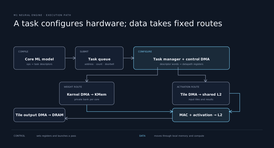
This split explains why a high-level model can be supported even when a particular hardware block lacks a programmable instruction set. The compiler can break work into supported passes, select memory layouts, and issue multiple descriptors. It also places a great deal of responsibility on the compiler. If a tensor does not fit the expected shape or movement pattern, software must rearrange it or use another compute unit.
Apple’s Core ML documentation describes a system that can use the CPU, GPU, and Neural Engine together. Its compute-unit choices let an app allow or exclude devices; allowing the ANE does not mean that every operation of a model runs there. The reverse-engineered task format is an implementation detail below that public API.
The memory hierarchy embodies a workload assumption
Unified memory means the CPU, GPU, and ANE can address the same system DRAM pool. It does not mean a multiply-add lane consumes operands directly from DRAM on every cycle. Yoon identifies a shared 2 MiB ANE L2 and, per core, a 64 KiB private kernel-memory bank plus input staging. Sixteen kernel banks amount to 1 MiB of dedicated weight storage.
There are separate transfer paths. A kernel DMA path brings weights from DRAM into each core’s private bank. A tile-input DMA path brings activations from DRAM into shared L2. A tile-output path sends results back. Intermediate tiles can remain in local memory between passes, and weights can remain near a core while many input positions pass through it.
Physical evidence supports this hierarchy. A firmware debug routine copies sixteen 64 KiB kernel-memory regions, one selected core at a time, and then one separate 2 MiB L2 region. On the die, Yoon maps compute cores around the central SRAM area. This layout shortens the routes from a shared tile store to many cores while keeping each core’s coefficients nearby. The exact internal arbitration remains unknown, but the storage capacities and visible paths agree with the behavior found in registers and benchmarks.
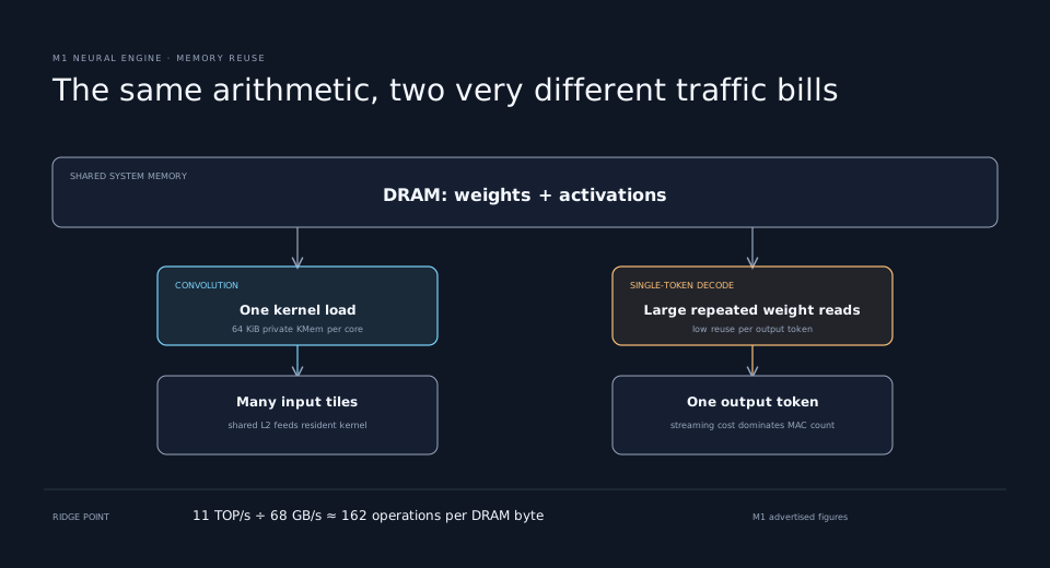
The roofline calculation makes the need for reuse concrete. One FP16 multiply-add counts as two arithmetic operations and reads two 2-byte operands. If both operands came fresh from DRAM, that would be only 0.5 operations per byte. Sustaining M1’s advertised 11 TOP/s at that rate would demand about 22 TB/s, far beyond its roughly 68 GB/s system-memory bandwidth. Dividing those two advertised figures gives a theoretical ridge point near 162 operations per byte of DRAM traffic. The number is a simplified ceiling, not a measured threshold for every model, but it shows why local reuse is the design’s central feature.
The asymmetry between kernels and tiles is especially revealing. Kernel storage has its own load-only route from DRAM. Yoon could not find a direct shared-L2-to-kernel-memory path. That observation is consistent with a design expecting coefficients to be loaded infrequently, remain private to a core, and be reused while activation tiles move. It is an excellent arrangement for many image convolutions. It is awkward when a value already in local tile memory needs to become the next operation’s coefficient. The absence of a path is evidence; the original designers’ intent is a plausible inference, not something the registers can prove.
The coefficient side exposes another constraint. Yoon found sixteen logical kernel-DMA lanes and measured tasks that made progress across them concurrently, but logical lanes do not prove sixteen fully independent physical engines. Requests can still converge on shared generation, crossbar, cache, and DRAM resources. More lanes help distribute weights to cores; they do not create more external bandwidth.
The distinction between weight memory and tile memory made sense for the convolution-heavy models common when Apple introduced its first Neural Engine in the A11 era. A filter is read-only during inference and reused at every spatial position, while activations change from tile to tile and intermediate outputs may become later inputs. Giving those operand classes different paths saves area and control complexity. The cost appears when newer models treat large, frequently streamed matrices as the dominant operand.
Why token decoding exposes the trade-off
Generating one token with a large transformer often requires reading most model weights for that token. With little reuse across a single step, speed is governed by sustained weight-streaming bandwidth more than by peak multiply-add count. This is where a machine built around small resident kernels meets a different workload shape.
Yoon measured bandwidth using large, data-dependent transfers and the slope of execution time as payload size increased. In that experiment, kernel DMA sustained 37.99 GB/s, tile DMA 59.08 GB/s, and a Metal GPU read test 77.70 GB/s. These are measurements for the author’s devices and workloads, not universal M1 specifications. A second experiment combined kernel and tile traffic. Runtime tracked the sum of the separate transfer times closely, suggesting the two read paths did not materially overlap in that setup. For a workload that must keep streaming both operands, a theoretical sum of their individual bandwidths is therefore misleading.
This also corrects a common shortcut in accelerator comparisons. “Both devices share unified memory” does not imply that they reach DRAM at the same rate. Request generation, transfer scheduling, local buffering, and contention still differ. Nor does a single throughput figure prove that one device is always faster: batch size, model shape, precision, compilation, and power limits can change the answer. The measurements identify a bottleneck for a particular decode-like pattern.
The M5 is an evolution, not a disappearance
The original research interprets newer GPU-based neural acceleration as a sign that the standalone NPU may be nearing its end. Apple’s own M5 announcement supports a narrower conclusion. M5 adds a Neural Accelerator to each GPU core and retains a faster, separate 16-core Neural Engine. The product now offers multiple places to run machine-learning work, each with different strengths. Apple has not announced the removal of the ANE.
The M1 investigation remains valuable precisely because newer hardware does not erase its lesson. Accelerator performance is not contained in the count of arithmetic lanes. It emerges from the whole route: model compiler, task launch, on-chip storage, transfer engines, operand reuse, and external bandwidth. The M1 ANE made a coherent bet that coefficients would stay near the compute cores while predictable activation tiles flowed through them. Reverse-engineering the path makes both the success of that bet and its limits visible.
For an engineer choosing where a model should run, the practical questions follow directly: How often are weights reused per output? Can intermediate tiles stay local? Which transfers overlap? What bandwidth does the actual compiled workload sustain? Answer those before comparing TOP/s. The memory traffic, not the multiplication, is often the story.