What does a ZIP file have in common with a language model? Both are in the business of guessing what comes next.

That sounds strange because their outputs look nothing alike. A compressor gives us a smaller file that can be reconstructed exactly. A language model gives us new tokens. Underneath those different jobs, however, sits the same useful object: a probability distribution over the next symbol.

Once we have those probabilities, an entropy coder can turn good guesses into short bit sequences. A likely symbol costs few bits. A surprising symbol costs many. Compression ratio therefore becomes a score for prediction quality—provided we count the model and its operating cost honestly.

This connection is more than a clever analogy. It explains why context improves compression, why cross-entropy is measured in bits, how a compressor can become a generator, and why a giant neural network is usually the wrong tool for shrinking an HTTP response.

Compression begins with redundancy

Lossless compression works because real data is rarely random. Source code repeats keywords and indentation. Logs repeat timestamps, field names, and service identifiers. English text has common letters, common words, and strong grammatical patterns. Images contain nearby pixels with related colors.

The simplest example is run-length encoding. A sequence such as:

AAAAAAAAAABBBBCC

can be described as ten As, four Bs, and two Cs. The description is shorter because the input contains long runs. But the same method makes ABCDABCD larger, not smaller. A transform only helps when it matches the structure of the data.

General-purpose compressors use richer structure. DEFLATE, the format behind gzip, combines LZ77 back-references with Huffman codes. Its back-references replace repeated byte sequences with a length and a distance, while its codes give shorter representations to frequent values. The DEFLATE specification allows a reference to reach up to 32 KiB into earlier input.

These techniques look different, but both exploit predictability. Repetition makes the next bytes easier to anticipate. Skewed frequencies make some symbols much safer guesses than others.

Separate the model from the coder

A helpful mental model divides a compressor into three parts:

1. A transform rearranges or describes the input so useful patterns become easier to see.
2. A probability model estimates how likely each possible next symbol is.
3. An entropy coder converts the real symbol and its estimated probability into bits.

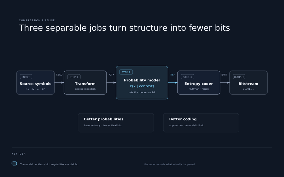
The boundaries are not always clean in production formats, but the split reveals where compression gains come from. Once an entropy coder is already close to the theoretical limit, improving the final coding trick offers little room. Improving the probability model can still reduce the limit itself.

Imagine a source with four possible symbols:

Symbol	Model probability
A	1/2
B	1/4
C	1/8
D	1/8

A sensible binary code uses one bit for A, two for B, and three each for C and D. Common events receive short paths; rare events receive long ones. This is the core idea behind Huffman coding.

The ideal information cost of an event with probability p is:

cost = -log2(p) bits

A probability of 1/2 costs one bit. A probability of 1/8 costs three. A probability of 1/1024 costs ten. Every time probability halves, the bill rises by one bit.

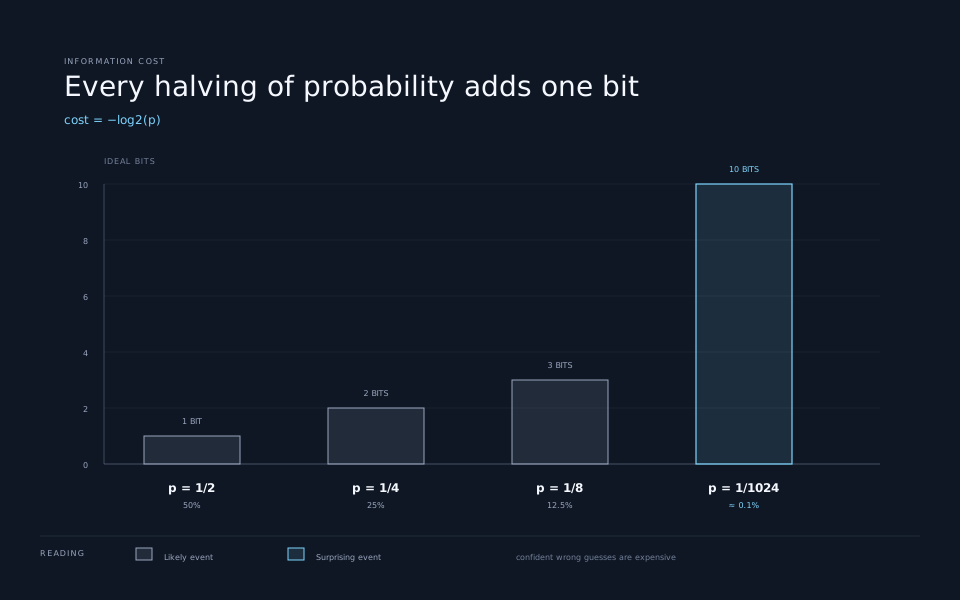
This formula gives prediction an exact price. A confident correct guess is cheap. A confident wrong guess is expensive.

Entropy is the average bill

Shannon entropy is the model’s expected number of bits per symbol:

H(P) = -Σ p(x) log2 p(x)

For the four-symbol distribution above, the average is 1.75 bits per symbol. A fixed-width code would need two bits because it must reserve equal space for four possibilities. A variable-length or arithmetic code can approach the lower average by spending fewer bits on common inputs and more on rare ones.

Entropy is not a universal property of a file detached from assumptions. It depends on the distribution used to describe that source. If we pretend every character is equally likely, we get one bound. If we know the language, file type, previous symbols, or document structure, we get another.

That is why there is no single best compressor. A model tuned for genomic sequences will see patterns that a generic byte model misses. A compressor for executable code can exploit structure that does not occur in photographs. The coder may be excellent in every case; the model decides which regularities are visible.

Arithmetic coding turns probabilities into ranges

Huffman coding assigns a whole-number count of bits to each symbol. That is fast and practical, but probabilities do not normally align to powers of two. A symbol with probability 0.7 has an ideal cost of about 0.515 bits, yet no standalone prefix code can give one symbol half a bit.

Arithmetic coding avoids that rounding problem by encoding a sequence as a position inside a range.

Start with the interval [0, 1). Divide it into sections whose widths match the symbol probabilities. If A has probability 0.7, its section occupies 70% of the interval. After reading the real next symbol, keep only that symbol’s section. Divide the remaining section again using the probabilities for the following symbol, then repeat.

For a sequence A B A, the interval narrows three times. At the end, any binary fraction that lands inside the final interval identifies the whole sequence, as long as the decoder has the same model and knows when to stop. More probable sequences preserve wider intervals, and wider intervals require fewer binary digits to identify.

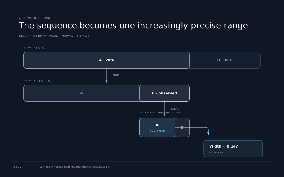
Practical implementations do not store an infinitely precise floating-point number. They maintain integer ranges, emit stable leading bits as the interval narrows, and renormalize continually. The elegant interval picture explains the mathematics; range coders and related techniques make it work on real machines.

The important point is not the specific coder. It is that the number of emitted bits tracks the model’s probability for the observed data.

Context makes a model useful

A table of global character frequencies is weak. In English, u is not especially common overall, but after q it becomes highly likely. In source code, ) may be ordinary globally but strongly expected after a function’s final argument. In a JSON document, a colon becomes likely after a closing quote in an object key.

An order-0 model ignores history. An order-1 model conditions its probabilities on the previous symbol. Higher-order models look at longer contexts:

P(next symbol)
P(next symbol | previous symbol)
P(next symbol | previous N symbols)

Longer context can sharpen predictions. If the actual next symbol receives more probability, its code becomes shorter. But simply storing a table for every possible context grows expensive and sparse. Most long contexts appear rarely, so estimates become unreliable.

Compression research has produced many ways to balance context and cost: backing off to shorter histories, mixing predictions from several models, updating counts online, and using learned representations rather than exact context tables. Modern language models are an extreme version of that search. They use a large parameterized model to turn a long token context into probabilities for the next token.

A language model already produces what a coder needs

During generation, a language model receives existing tokens and returns logits, which are converted into probabilities. A sampling rule chooses a token, appends it, and repeats.

Compression changes only the choice step. The encoder already knows the real next token because it is reading the source document. It asks the model for probabilities, looks up the probability assigned to that real token, and sends the token through an entropy coder. The decoder runs the same model on the reconstructed context and uses the coded bits to recover which token came next.

The loop is deterministic:

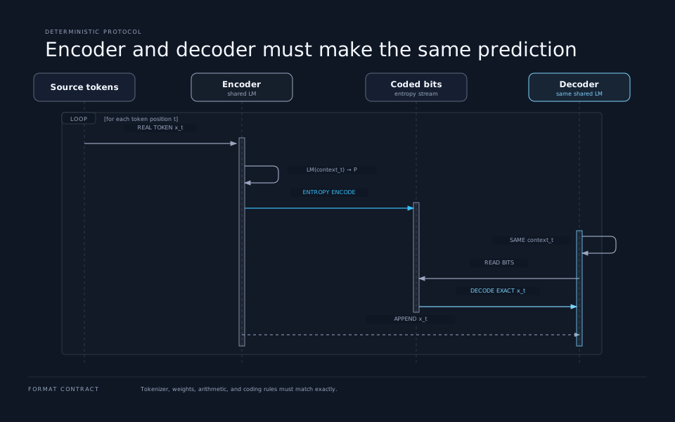
Both sides must use exactly compatible tokenization, model weights, arithmetic, and coding rules. A tiny disagreement changes later context, which changes later probabilities, and the entire reconstruction diverges. Reproducibility is therefore part of the format, not an implementation detail.

The connection also explains the standard training objective. Cross-entropy measures the average negative log probability assigned to real next tokens. When logarithms use base two, the unit is bits per token. Reducing language-model loss means assigning more probability to the observed data; in coding terms, it means describing that data with fewer bits.

Google DeepMind’s Language Modeling Is Compression makes the equivalence operational. The researchers evaluated language models as general-purpose compressors and also reversed the direction, using ordinary compressors to build conditional generative models. Their results connect scaling, tokenization, in-context learning, prediction, and code length under one measurement.

A compressor can generate, too

The relationship runs both ways. A compressor implicitly defines probabilities over continuations: data that it can encode cheaply is data it considers unsurprising.

Suppose we want to compare candidate continuations after a prompt. Append each candidate, compress the result, and observe the extra code length. The continuation that adds the fewest bits is, in a rough sense, the one the compressor predicts best. With the right construction, these code-length differences can be normalized into a probability distribution and sampled.

This does not turn gzip into a strong conversational model. Its short sliding window and byte-level pattern matching capture local repetition, not rich semantic structure. But it demonstrates that generation and compression are not separate species of computation. They are two ways of using a model’s probability distribution:

• Compression follows the observed data and records the choices efficiently.
• Generation samples choices from the model and creates new data.

Why we do not ship an LLM with every archive

If a neural model predicts well, why not replace gzip everywhere? Because compressed size is only one line in the cost ledger.

The decoder needs the model. When sender and receiver do not already share it, model weights are part of the total description. A multi-gigabyte predictor is absurd overhead for a 100 KiB web response. Even for a huge corpus, the compute and memory needed for token-by-token inference may dominate the storage saved.

Real compression systems optimize several constraints at once:

• compressed size;
• encoding and decoding speed;
• peak memory;
• random access and streaming behavior;
• model or dictionary distribution;
• deterministic portability;
• error recovery and format longevity.

HTTP compression prizes fast, tiny decoders that are already installed in browsers. Backups may accept slower encoding for smaller long-term storage. Satellite links may justify a shared domain model because every transmitted bit is costly. Archival formats may reject a learned model if reproducing its runtime decades later is uncertain.

There is also a crucial accounting distinction. If a pretrained model is already present for another reason, its marginal cost may be close to zero. If the compressed artifact must be self-contained, the model cost cannot be ignored. Claims of spectacular neural compression often depend on which side of that boundary the weights occupy.

Compression is an honest model test—with conditions

Prediction benchmarks can be distorted by sampling settings or subjective evaluation. Lossless compression supplies a hard score: reconstruct the input exactly and count the bits. A model that assigns better-calibrated probabilities to the real sequence earns a shorter code.

But the score answers a narrow question. It measures how well a probability model fits a data distribution after accounting for the agreed coding setup. It does not, by itself, prove reasoning, factuality, usefulness, or understanding. A compressor can exploit syntax in a language its designer cannot read. A language model can predict fluent text while being wrong about the world.

Fair comparisons must also include:

• the model or dictionary size;
• tokenizer and metadata overhead;
• the precision and determinism requirements;
• compute used by both encoder and decoder;
• whether training data overlaps the test set;
• performance on data outside the expected distribution.

These conditions do not weaken the connection. They keep us from turning a precise mathematical equivalence into a vague claim about intelligence.

The practical lesson: improve the probabilities

When an entropy coder is already efficient, better compression comes from finding a better description of the source.

That might mean a transform that exposes repetition, a dictionary shared by both endpoints, a context model specialized for the file type, or a learned predictor for a large and valuable dataset. It might also mean choosing a simpler model because its speed and portability beat a small gain in ratio.

The most useful way to think about a compressor is therefore not as a machine that squeezes bytes. It is a machine that makes a sequence of probabilistic bets and then writes down what actually happened. Good bets are cheap to record. Bad bets are expensive.

Language models make the same bets before choosing their next tokens. The machinery around them is newer and much larger, but the bill still arrives in bits.

Further reading

• Compression is prediction, Annie Sexton’s interactive walkthrough of models, arithmetic coding, entropy, and LLMs.
• Language Modeling Is Compression, the full DeepMind research paper.
• DEFLATE Compressed Data Format Specification, the format behind gzip’s compression method.
• Arithmetic coding, a compact definition from NIST’s Dictionary of Algorithms and Data Structures.