Decision Trees: Why Nested Rules Still Matter in the LLM Era
On March 3, 2026, one of the top stories on Hacker News was Decision trees – the unreasonable power of nested decision rules (id=47213219). At drafting time, the story had 539 points and 80 comments, making it one of the most active technical discussions on the front page.
The article is from Amazon’s MLU Explain project, a visual explainer series for machine learning concepts. This particular installment covers decision trees from first principles: what they are, how they learn, where they break, and what to do about it. The HN thread landed because engineers in 2026 still encounter these questions regularly, and the interactive visuals make the concepts click faster than a textbook derivation.
Here is a full walkthrough of the ideas, with the math and intuitions that the original article builds toward.
What a Decision Tree Actually Is
A decision tree is a supervised machine learning algorithm that makes predictions by routing data through a series of yes/no questions. Visually, it looks like a flowchart: each internal node tests a feature, each branch is a possible outcome of that test, and each leaf node holds a final prediction.
The core claim of the original article—the “unreasonable power” in the title—is that this simple architecture, just nested if/else rules, can model surprisingly complex patterns while remaining completely inspectable. Every prediction has an audit trail you can trace from the root to the leaf.
Decision trees handle both classification (predicting a discrete category) and regression (predicting a continuous value). The mechanics are the same; only the leaf labeling changes.
Building a Tree: The Running Example
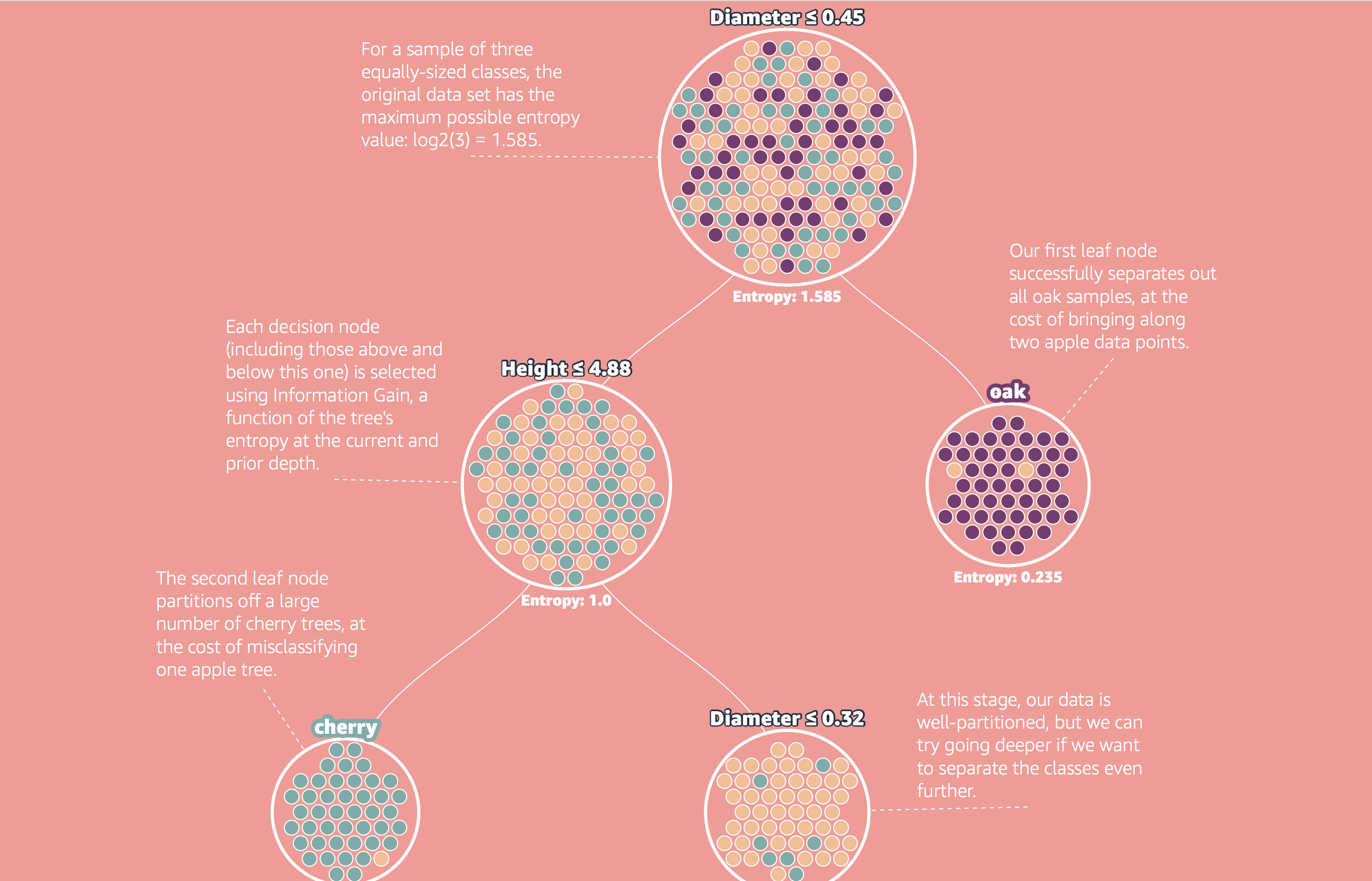
The article walks through a concrete classification problem: given a dataset of trees with two features, trunk diameter and height, predict the species—Apple, Cherry, or Oak.
The finished tree uses four splits:
- Diameter ≥ 0.45 at the root → routes Oak trees to the right
- Height ≤ 4.88 → separates Cherry trees below
- A further horizontal split on height → partitions remaining Apple and Cherry trees
- A final split → completes the classification for ambiguous examples
Each split carves the feature space into rectangular regions. After enough splits, each region is dominated by one class, and the leaf label becomes the majority class in that region.
The key question is: how does the algorithm decide which feature to split on, and where to cut it? That is where entropy comes in.
Entropy: Measuring Disorder
Entropy, borrowed from information theory, measures how uncertain or mixed a dataset is. If every example in a node belongs to the same class, entropy is zero—there is no uncertainty left, and no further splitting is needed. If examples are evenly distributed across all classes, entropy is at its maximum.
The formula is:
H = -∑ p_i * log₂(p_i)where p_i is the proportion of examples belonging to class i. The log base 2 gives entropy in bits.
Two boundary cases are worth anchoring on:
- Pure node: one class holds everything, so
p_i = 1for that class and 0 for all others. Each term is either-(1 * log₂(1)) = 0or-(0 * log₂(0)) = 0by convention. Entropy = 0. - Maximum confusion: for two classes split 50/50, entropy =
-(0.5 * log₂(0.5)) * 2 = 1 bit. For three equally likely classes, entropy ≈ 1.585 bits.
Entropy gives you a single number that tells you how much work is left to do at a node. The algorithm’s job is to pick splits that reduce this number as quickly as possible.
Information Gain: Picking the Best Split
Information gain measures how much entropy drops when you split the data on a particular feature at a particular cutoff. The formula is:
IG = H(parent) - ∑ (|child_k| / |parent|) * H(child_k)In plain terms: start with the parent’s entropy, subtract the weighted average entropy of the two child nodes after the split. The weights are the fraction of examples going to each child. A larger information gain means the split does a better job separating the classes.
The algorithm tests every possible split candidate—every feature, every threshold—and picks the one that maximizes information gain. In the Apple/Cherry/Oak example, the article shows this search over the Diameter feature, with peak information gain of 0.574 at Diameter = 0.45. That is why the root node splits there and not anywhere else.
After placing that first split, the algorithm recurses: each child node becomes a new subproblem, and the same entropy/information gain calculation runs again on the subset of data that reached that node.
The ID3 Algorithm
The procedure has a name: ID3 (Iterative Dichotomiser 3), one of the earliest and most studied decision tree algorithms. The full sequence is:
- Compute entropy for the current node’s dataset.
- For every feature and every possible threshold, compute the information gain of splitting there.
- Select the split with the highest information gain. Create an internal node for it.
- Recurse on each child subset.
- Create a leaf node when a stopping condition is met: the node is pure (entropy = 0), no features remain to split on, or a user-specified constraint is hit (maximum depth, minimum examples per leaf).
- Label each leaf with the majority class (for classification) or the mean value (for regression).
The result is a tree that partitions the training data until every region is either pure or stopped by a constraint. Left unconstrained, ID3 will keep splitting until it perfectly fits the training set—which is exactly where the problems begin.
Overfitting: When the Tree Learns Too Much
A fully grown decision tree memorizes the training data. Every quirk, every outlier, every bit of measurement noise gets encoded into a split somewhere. The tree achieves near-perfect training accuracy, but its test accuracy often collapses. This is the classic overfitting failure mode.
The connection to the bias-variance tradeoff is direct:
- High bias: a tree with too few splits makes oversimplified predictions. It underfits—it misses real patterns in the data.
- High variance: a tree with too many splits fits noise. It overfits—it learns the training set, not the underlying distribution.
The depth of the tree is the primary control over this tradeoff. Shallow trees have high bias and low variance; deep trees have low bias and high variance. The goal is a depth that balances the two on held-out data.
Regularization strategies that ID3 variants typically expose:
- Maximum depth: hard cap on how deep the tree can grow. Forces early stopping.
- Minimum samples per split: refuse to split a node unless it contains at least N examples. Prevents hair-trigger splits on small groups.
- Minimum samples per leaf: ensure each leaf has at least N examples. Avoids leaf nodes that represent single training points.
These hyperparameters are tuned through cross-validation. The interaction between them is nonlinear, so a grid search or random search over small ranges tends to find a good operating point faster than manual tuning.
Variance and Instability: The Deeper Problem
Even a well-regularized single tree has a structural problem that overfitting regularization does not fully solve: high variance.
The article demonstrates this with a striking experiment. Take the same training set, add tiny random Gaussian noise to just 5% of the examples, and retrain the tree. The resulting tree structure often looks completely different from the original. Different splits, different depths, different leaf assignments.
This happens because decision trees make greedy, hard-boundary decisions at each node. A slightly different data point near a split boundary can flip which feature and threshold are chosen. That flip cascades down the tree, changing everything below it. Small input changes produce large structural changes.
High variance means the model is unstable. You cannot trust a single tree to reliably represent the patterns in your data—you can only trust what it happened to find for this particular training sample.
Gini Impurity: An Entropy Alternative
Before addressing variance at the algorithmic level, one variation worth knowing: Gini impurity. It is an alternative to entropy for measuring node disorder, defined as:
Gini = 1 - ∑ p_i²Like entropy, Gini is zero when a node is pure (one class has probability 1, so 1 - 1² = 0) and increases as the class distribution becomes more mixed. The maximum for two classes is 0.5.
Gini impurity avoids the logarithm, so it is cheaper to compute. In practice, trees built with Gini and trees built with entropy produce comparable results, with measurable differences mainly on imbalanced datasets. Most production implementations (scikit-learn, XGBoost, LightGBM) default to Gini for classification. The choice rarely dominates other hyperparameter decisions.
Random Forests: Trading Variance for Reliability
The standard answer to decision tree variance is the random forest, introduced by Leo Breiman in 2001. The mechanism is straightforward:
- Bootstrap sampling: draw N training sets from the original data by sampling with replacement. Each sampled set is roughly 63% unique examples from the original, with the rest duplicated.
- Feature subsampling: at each split, only consider a random subset of features (typically
√num_featuresfor classification). This decorrelates the trees. - Train one full tree on each bootstrapped set, using the feature subsampling rule.
- Aggregate predictions: for classification, take the majority vote across all trees. For regression, take the mean.
Each individual tree still overfits its bootstrapped training set. But because the trees are trained on different data samples and make decisions on different feature subsets, they overfit in different directions. Their errors are uncorrelated, so averaging them out cancels the individual mistakes.
The result is a model with substantially lower variance than any individual tree, at the cost of losing interpretability—you can no longer trace a single prediction through a single decision path.
Random forests also produce a useful side benefit: out-of-bag error estimation. Because each tree sees only ~63% of the training data, the held-out examples can be used to estimate test error without a separate validation set. This makes hyperparameter tuning cheaper.
Breiman’s original paper, Random Forests (2001), remains worth reading as the canonical reference. It establishes the theoretical foundations and empirical benchmarks that subsequent ensemble methods still cite.
Why This Combination Still Matters in 2026
The MLU Explain article is fundamentally an argument that decision tree fundamentals are not obsolete—they are load-bearing concepts for anyone working with tabular data or building interpretable systems. That argument holds for a few concrete reasons.
Structured data is everywhere and different from images and text. Foundation models trained on unstructured data do not transfer easily to tabular features with mixed types, missing values, and domain-specific distributions. Tree-based methods were designed for exactly this structure and still dominate structured data benchmarks.
Gradient-boosted trees are the direct descendants. XGBoost, LightGBM, and CatBoost—the models that regularly win Kaggle competitions on tabular data—are all built on the same split-selection logic as ID3. Understanding entropy and information gain gives you the foundation for understanding why these tools work and how to tune them.
Interpretability is a design constraint, not a nice-to-have. For fraud detection, credit scoring, healthcare risk prediction, and compliance-sensitive ML, model decisions must be explainable to regulators, auditors, or end users. A single decision tree with a reasonable depth budget delivers a prediction plus a readable proof. That combination is not replicated by most black-box alternatives.
Engineering Guidance for Teams Building with Trees
Use Trees First for Tabular Baselines
Before reaching for a neural network or a large pretrained model for a structured data problem, build a regularized single tree and then a random forest or gradient-boosted tree. These steps cost hours, not days, and give you:
- A performance floor to beat
- Feature importance scores that help domain experts sanity-check the model
- A fast debugging surface when predictions look wrong
Tune Depth and Regularization Before Architecture
The single-tree hyperparameters that matter most are maximum depth, minimum samples per leaf, and (for ensembles) number of estimators and subsampling rate. Tuning these with cross-validation before switching to a more complex model family is almost always worth doing first.
Treat Feature Importance as a Hypothesis Generator
Tree-based feature importance (measured by total information gain attributed to each feature across all splits) is fast to compute and interpretable, but it is biased toward high-cardinality features and can be misleading for correlated inputs. Use it to generate hypotheses, then validate important features using permutation importance or SHAP values before acting on them.
Know When to Move to Ensembles
A single tree at optimal depth will plateau. When cross-validated performance stops improving with more depth, that is the signal to move to a random forest or gradient-boosted ensemble. The jump in performance is usually significant. The jump in complexity is manageable if the team already understands the underlying tree mechanics.
Closing
Decision trees are a useful corrective to “newer must be better” thinking. The ideas that the MLU Explain article covers—entropy, information gain, the bias-variance tradeoff, variance reduction through ensembles—are the same ideas powering the highest-performing tabular ML systems today. They just wear different names in different frameworks.
In 2026, with increasingly complex AI stacks, understanding these foundations from first principles is a competitive advantage. Not because you will train decision trees on every problem, but because you will understand what the systems doing the training are actually doing.
Canonical References
- MLU Explain: Decision Trees — the visual explainer this post is based on, from Amazon’s Machine Learning University
- Scikit-learn: Decision Trees — production-grade API reference with strengths, limitations, and regularization controls
- Breiman (2001): Random Forests — the foundational paper for bagged tree ensembles and out-of-bag error estimation