A drone photograph shows a tiny tropical resort, two neighboring islands, open ocean, and no readable sign. The file contains no useful EXIF metadata. There is no GPS position, camera height, lens record, or convenient landmark. Taken literally, the question “where is this?” appears to ask for visual recognition across every island on Earth.

It can be made into a search problem instead.

The photograph does not reveal absolute distances, but it does preserve a rough arrangement: one very small cay sits near two larger landmasses; the lines from the cay to its neighbors form a particular angle; one neighbor appears farther away than the other; one has elevated terrain; and a broad side of the triangle opens onto water. These relationships are noisy, yet they are distinctive enough to become a fingerprint.

That idea powered a remarkable solution to Gralhix OSINT Exercise #004. The solver, Yasser, converted a visual hunch into geometry, tested tens of millions of island triples with CUDA, and then used Sentinel-2 vegetation data and Copernicus elevation tiles to reduce the survivors. The answer was Oan Resort in Micronesia, near 7.363444° N, 151.755750° E, with the camera facing roughly northwest.

The interesting part is not simply the answer. It is the architecture of the search: preserve scale-resistant evidence, use uncertainty bands instead of false precision, order filters by cost, and reserve human inspection for a final list small enough to understand.

Start by refusing the easy answer

Reverse-image search can solve many geolocation puzzles in seconds. That is useful when the goal is to identify the place. It is less useful when the goal is to learn what the image itself contains.

Here the deliberate constraint was to avoid visual lookup and build the answer from public geographic data. The source image was a 736 by 515 lossless WebP with no helpful metadata. Without camera height and calibration, a rigorous reconstruction of ground distances from pixels was not available. Perspective also means that a length measured in the image is not automatically proportional to a length on the surface.

Rather than pretend otherwise, the method kept only approximate relationships.

Three clicks marked the visible landmasses:

• P0: the tiny resort cay;
• P1: the larger island on the right;
• P2: the mountainous island toward the left/front.

A small desktop tool recorded the pixel coordinates. From those points it calculated the angle at P0 and the ratio between the two sides extending from P0. Each measurement received a tolerance of about 20 percent. This is a key choice: the clicks are observations made through perspective, not survey data. A window acknowledges that uncertainty while remaining selective.

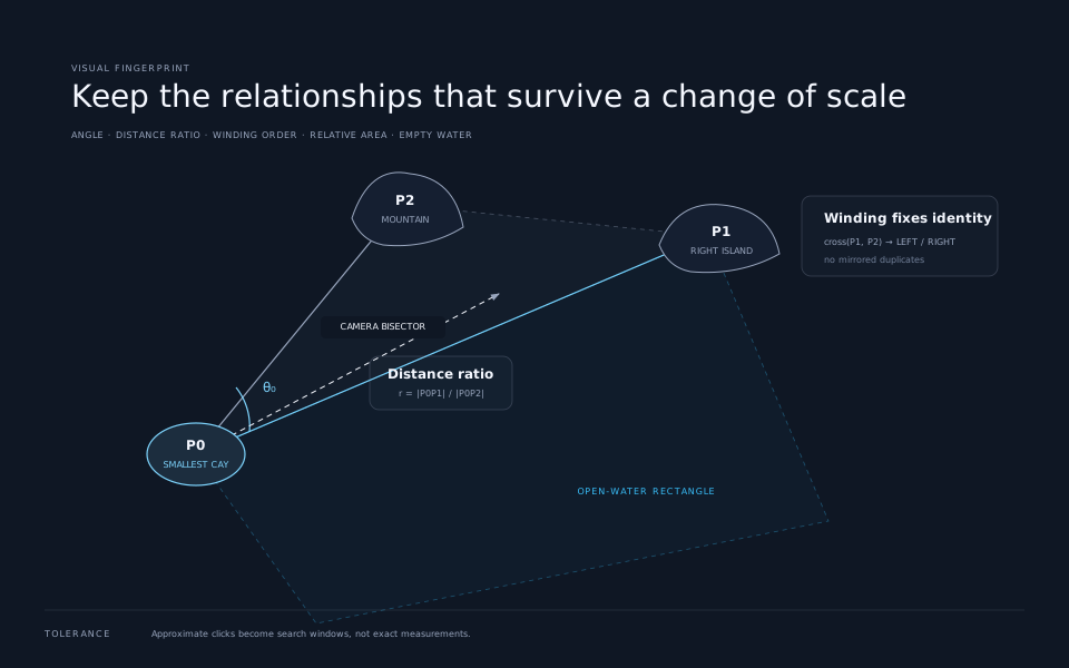
The triangle needs an orientation as well as three lengths. If the two larger islands can be swapped freely, mirrored arrangements create duplicate candidates. A two-dimensional cross product supplies a consistent winding order:

cross = ax × by − ay × bx

The sign says whether the turn from one vector to the other is clockwise or counterclockwise. That lets every candidate assign P1 and P2 the same way before comparing angles and ratios.

The smallest landmass was also expected to be P0. Relative polygon area therefore becomes another test. None of these clues is decisive alone. Together they define a searchable signature.

Turn the planet into candidate points

The global input was OpenStreetMap’s split land-polygon dataset in WGS84 coordinates, about 882 MB. Each polygon represents land; its geometry supplies an area, perimeter, outline, and a representative position.

A naive approach would compare every possible triple of land polygons. That is impossible in practice because combinations grow as:

C(n, 3) = n(n − 1)(n − 2) / 6

The solution is to make the candidate universe smaller before generating triples.

The photograph looks tropical, so the first filter keeps latitudes between −30° and +30°. This is not a theorem. It is an explicit prior derived from the sky, vegetation, shallow water, and resort setting. It leaves 141,131 land polygons.

Next comes local density. For each candidate, count nearby centroids within five kilometers. More than ten neighbors suggests a dense reef field, crowded coastline, or large archipelago unlike the sparse scene in the photograph. This reduces the set to 51,576 points.

The remaining points are grouped with a cKDTree. A point must have at least two neighbors within 20 kilometers, because the image requires a three-landmass arrangement. This produces roughly 23,500 local clusters.

Only then does the method enumerate triples. A cluster of 60 points already contains 34,220 combinations. To stop unusually dense clusters from dominating memory, each cluster is capped at 60 members using a stratified sample: one third from small polygons, one third from large polygons, and one third from the middle of the area distribution. That is more faithful to the expected mix than a purely random sample.

After expansion, the search contains 80,690,777 candidate triples.

Why the GPU is the right tool here

Eighty million sounds alarming until the work per item is examined. Every candidate performs the same compact calculation over independent data:

1. Sort three polygon areas to identify the smallest landmass as P0.
2. Use the cross-product sign to assign P1 and P2 consistently.
3. Calculate two displacement vectors from P0.
4. Compare the angle at P0, distance ratio, relative areas, and side-length windows with the photographic fingerprint.
5. If all masks pass, append the triple to an output array.

This is the shape CUDA handles well: a very large number of independent, regular tests with little shared state. The implementation launches one thread per triple. Passing threads claim an output slot with an atomic counter, so simultaneous hits do not overwrite one another.

On an NVIDIA RTX 3050, the reported kernel processed the 80.7 million triples in about 204.1 milliseconds and produced 158,784 raw matches. The impressive number should be read correctly. It is kernel time for the parallel matching stage, not the duration of loading 882 MB of vectors, preprocessing polygons, generating combinations, transferring arrays, calling remote services, or tuning heuristics. GPU acceleration removes one computational bottleneck; it does not make the entire investigation instantaneous.

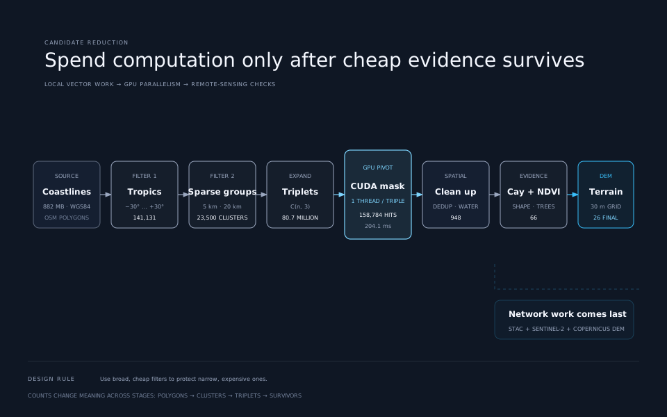
The raw match count also contains duplicates because one physical triple can belong to several overlapping clusters. Deduplicating by the ordered identity (P0, P1, P2) leaves 8,915 unique triples.

Empty space is evidence

Object matching usually asks what is present. This search also asks what must be absent.

The source photograph contains open water on the side of the P0 → P1 edge opposite P2. For every surviving triple, the method constructs a rectangle extending into that side and checks it against the land dataset. If another polygon intersects the rectangle, the arrangement is inconsistent with the unobstructed ocean in the image.

That negative-space test cuts 8,915 triples to 948.

It is a broadly useful pattern. A skyline can be identified by gaps between buildings. A road scene can be constrained by the absence of intersections. A network incident can be narrowed by expected events that never occurred. When a scene has strong empty regions, encode them instead of treating them as background.

Test whether the tiny island looks like a cay

The next filters look at the outline and neighborhood of P0.

First, the Polsby–Popper compactness score compares area with perimeter:

compactness = 4π × area / perimeter²

A perfect circle scores 1; jagged or elongated shapes score less. Candidates below 0.5 are discarded because the visible resort resembles a compact coral cay.

Second, a “micro-cay halo” test looks for at least one land fragment smaller than 0.05 km² within 1.5 kilometers. Reef systems often scatter tiny sandbars and fragments around the principal cay. Requiring one nearby fragment, together with compactness, leaves 213 of the 948 candidates.

A minimum rotated rectangle then captures the island’s overall oval shape. Two values matter:

• The long-to-short aspect ratio must fall between 1.05 and 2.2.
• The polygon must fill enough of its bounding rectangle.

An ideal ellipse occupies π/4, or about 0.785, of its minimum bounding rectangle. The filter asks a real coastline to retain at least 75 percent of that ideal, giving a floor near 0.589. This rejects crescents, rings, deeply notched islands, nearly circular blobs, and very long slivers while keeping plausible solid ovals. The list falls to 137.

These thresholds are engineered heuristics, not definitions of a coral cay. Their value comes from being inspectable and cheap. Each states what visual belief it encodes, and each can be relaxed or replaced if it removes the true answer.

Ask satellite data only after geometry has done its job

Remote calls are slower and less predictable than local vector arithmetic, so satellite evidence arrives late in the pipeline.

The method queries Earth Search, Element 84’s public STAC API over open datasets on AWS. For each P0, it finds a recent Sentinel-2 scene with low cloud cover and samples the red and near-infrared bands. The normalized difference vegetation index is:

NDVI = (NIR − Red) / (NIR + Red)

Healthy vegetation usually reflects much more near-infrared than red light, while water and bare sand remain near zero or negative. Requiring NDVI above 0.6 looks for the dense tree cover visible on the resort cay. Sixty-six candidates survive.

The final automated check uses the Copernicus DEM GLO-30, a global digital elevation model distributed as cloud-optimized GeoTIFFs at roughly 30-meter spacing.

The bearing from P0 to both neighboring islands is calculated with spherical trigonometry. The bisector of those bearings approximates the camera’s forward direction. From that heading, the method sweeps a fan of sample points ±50° across distances from 2 to 20 kilometers.

Two conditions express the scene:

• P0 should remain at or below 50 meters, consistent with a low reef cay.
• Terrain in the forward arc should reach at least 100 meters but no more than 500 meters, matching a visible nearby mountain rather than a flat atoll or enormous peak.

Twenty-six candidates remain. At that size, an HTML report with country labels and satellite-map links is better than another fragile automatic classifier. Human inspection finds the matching geometry at the eighth row: Oan Resort in Chuuk, Federated States of Micronesia.

Using the recovered coordinates, the bearing from the cay toward the right-hand island is about 324.97°, which corresponds to northwest and answers the camera-direction part of the exercise.

What this method proves—and what it does not

The result is convincing, but the pipeline is not a general guarantee that any island photograph can be geolocated.

Several approximations matter:

• Pixel geometry is distorted by perspective, camera tilt, unknown altitude, and unknown lens parameters.
• Polygon centroids simplify irregular land shapes and can fall in unintuitive places.
• Treating degrees as roughly 111 km is a local approximation; longitude scale changes with latitude.
• OpenStreetMap coverage and polygon boundaries are not perfectly uniform worldwide.
• Cloud, acquisition date, shoreline movement, and pixel placement affect NDVI.
• A 30-meter elevation grid can miss narrow peaks or mix coastal land with water.
• Hand-tuned thresholds can overfit the particular scene and may exclude the correct answer in another puzzle.

For production geodesy, an ellipsoidal model such as WGS84 and a library like GeographicLib provides robust inverse-distance and bearing calculations. For this search, most comparisons occur over short distances in the tropics, where simpler local approximations are fast and the tolerance windows dominate small model errors.

The HN discussion also connected the terrain-matching idea to older navigation techniques such as terrain contour matching. The family resemblance is real: both compare observed terrain structure with a stored geographic model. The purposes and sensing systems differ, but the deeper strategy—navigate by matching shape when direct positioning is unavailable—predates modern satellite navigation.

The reusable engineering pattern

This investigation works because it treats uncertainty as a design constraint rather than an inconvenience.

First, convert qualitative observations into measurable features. “Tiny resort beside two islands” becomes relative area, a triangle angle, a side ratio, winding order, open water, vegetation, and terrain height.

Second, attach honest tolerance to weak observations. An approximate click should produce a search window, not six decimal places of confidence.

Third, order tests by cost and selectivity. Latitude, density, and local clustering are cheap. GPU arithmetic is expensive in volume but regular and local. Network-bound satellite and elevation checks are saved for the end.

Fourth, use the machine where the work is uniform and the human where ambiguity remains. CUDA is excellent at applying one mask 80.7 million times. A person is excellent at comparing 26 satellite scenes and recognizing the exact coastal arrangement.

Finally, keep the search explainable. Every stage has a reason, a threshold, an input count, and an output count. That makes failures debuggable. If the true island disappears, there is a concrete place to widen the search rather than a single opaque score to distrust.

The final coordinate is satisfying, but the durable lesson is larger: a photograph can become a database query when its visual relationships are translated carefully enough.

Sources and further reading

• Geolocating Random Islet Image Using Geometry & CUDA GPU Programming, the original technical walkthrough and results.
• Source code and generated reports, including the geometry, CUDA, satellite, and elevation stages.
• Hacker News discussion, including observations about camera calibration and terrain contour matching.
• Earth Search STAC API, used to discover Sentinel-2 imagery.
• Copernicus DEM on AWS Open Data, the elevation source used for the mountain check.
• Geodesics on an ellipsoid, a rigorous reference for distance and bearing calculations on WGS84.