Fast text-to-speech is easy to describe badly. A system can generate a minute of audio in less than a minute and still feel slow in conversation. It can return bytes quickly while those bytes contain silence. It can produce the first syllable promptly, then starve the player halfway through the sentence. It can look excellent with one request and collapse when several users arrive together.

Real-time speech therefore needs more than a fast model. It needs a serving system that understands when audio becomes audible, how much playable audio is buffered, which stage of the model is blocking a deadline, and how to share a GPU without turning every request into a long queue.

Nari Labs demonstrated that distinction with an open implementation of Qwen3-TTS 1.7B CustomVoice. On one NVIDIA H100 SXM, its latency-oriented profile sustained 10 requests per second while keeping p95 time-to-first-audio below 50 milliseconds and avoiding playback underruns. The important achievement is not one isolated kernel trick. It is the way measurement, scheduling, batching, graph capture, and state reuse reinforce one another.

This is the engineering pattern behind that result—and a useful template for other streaming generative systems.

“Real-time” has four separate requirements

The first metric is audible time-to-first-audio, or audible TTFA: the interval from dispatching a request until the client receives samples containing sustained sound. That last word matters. Time to first byte can stop when a response header or silent PCM arrives. Audible TTFA stops when a listener could actually hear speech.

The second requirement is continuity. Once playback starts, the next chunk must arrive before the buffered audio runs out. A 40 ms start followed by a 300 ms gap is worse than a smooth 120 ms start. Streaming systems need to track underruns, not just startup latency.

The third requirement is capacity. Results at one request per second say little about an interactive service. Queueing delay grows nonlinearly as utilization approaches the device’s limit, so p95 latency under an open stream of arrivals is more informative than a single sequential benchmark.

The fourth requirement is valid speech. Aggressive trimming, chunking, or decoding can make output malformed while still producing attractive latency numbers. Nari’s benchmark reconstructed received PCM and ran speech-to-text over completed output as a basic intelligibility check.

Together, these requirements define useful performance:

• low p95 audible TTFA;
• no playback underruns;
• stable behavior as request rate rises;
• intelligible, correctly formed output.

Any test that omits one of them creates an optimization escape hatch.

Measure the sound a user hears

Many TTS engines emit tens of milliseconds of leading silence. If a client starts its timer when the first PCM packet arrives, that silence makes the system look faster than it feels.

A more honest harness examines short windows of the waveform. Root-mean-square amplitude is a simple onset signal: compute energy over successive windows, require it to remain above a threshold long enough to reject tiny spikes, and record the first sustained speech sample. This produces an audible TTFA rather than a transport TTFA.

The same detector can trim leading silence before streaming. In Nari’s tests, dynamic trimming improved audible TTFA by roughly 80 ms for some engines. It did not accelerate inference; it removed a delay between generated data and perceived speech. That distinction should remain explicit in reports.

The arrival process matters too. Closed-loop tests send a request, wait for completion, then send another. They suppress queue formation and can make an overloaded service look healthy. Nari instead used five-minute open-loop runs with Poisson arrivals. Requests continue to appear independently of completion, which better exposes the latency tail a public endpoint will face.

The benchmark should also record every chunk’s arrival time and duration. If a chunk contains 160 ms of playable audio, the following chunk has about 160 ms to arrive after playback begins. That is a deadline, not a general command to run as fast as possible.

Qwen3-TTS is three different workloads

Qwen3-TTS uses a discrete multi-codebook speech representation. For each audio frame, the serving path has three main jobs:

1. The Talker predicts the first codebook token.
2. The Code Predictor autoregressively produces the other 15 codebook tokens.
3. The causal Codec converts those tokens into waveform samples.

These stages do not have the same shape. The Talker resembles language-model token generation. The Code Predictor executes a short, fixed-depth loop. The Codec combines transformer context with convolutional state and produces chunks of continuous audio. Their batch sizes, cache needs, execution lengths, and user-visible deadlines differ.

A conventional split deployment often groups Talker and Code Predictor work in one engine and runs the Codec in another. That permits some overlap, but it divides scheduling authority. One process cannot always see that a codec job is about to starve playback while another process is starting a long unit of predictor work.

Nari exposes all three modules as independently schedulable tasks on one scheduling surface. The scheduler chooses both the request to advance and the stage to run. It can prioritize a new request waiting for first audio, rescue an established stream nearing its playback deadline, and fill the rest of a batch with compatible work.

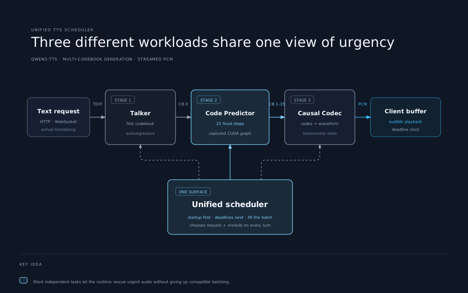
This is a general systems lesson. Separating work is valuable only when the pieces remain coordinated. A boundary that enables overlap can also hide urgency and create non-preemptible blocks.

Startup urgency and playback urgency are different

Before the first audible chunk, every millisecond is user-visible. The request should take a fast path through Talker, Code Predictor, and enough Codec work to begin playback.

After playback starts, the objective changes. Generating the next chunk immediately is often wasteful: the listener cannot consume it until the current buffer plays. The chunk only needs to arrive before its deadline. Work with more slack can yield GPU time to a request still waiting for its first sound.

This gives the scheduler two priority classes:

• startup-critical work, which has not produced audible audio;
• deadline-critical work, whose playback buffer is close to empty.

Everything else has slack. The scheduler can use that slack to build efficient batches.

Choosing urgent work alone would protect latency but waste the GPU on tiny batches. Nari uses the urgent request as an anchor, then adds compatible tasks to fill the remaining batch slots. The urgent item determines what must run now; opportunistic items make that turn economically useful.

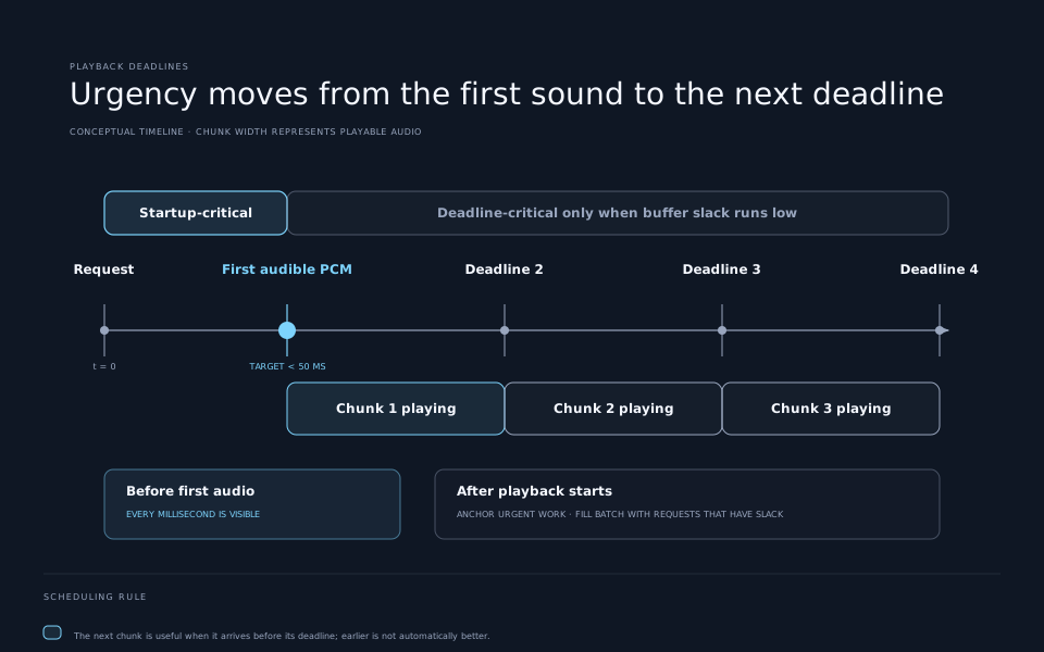
This approach resembles real-time scheduling more than ordinary throughput batching. The scarce resource is not simply GPU time. It is GPU time before a particular user-visible deadline.

Make the first chunk small, then grow it

Codec chunk size creates a direct trade-off. Small chunks reach the client quickly, but they provide little playback headroom and force more frequent decoder work. Large chunks batch efficiently and build a safer buffer, but delay the first audible sample.

The useful answer is a ramp:

• decode a small first chunk to minimize startup delay;
• increase later chunk sizes once playback has begun;
• tune the ramp against measured underruns and load, not intuition.

The same principle appears in the Codec implementation. Initializing incremental state has a fixed cost that hurts the startup path. Nari performs a full decode for the first audio, then switches to state-cached incremental decoding for later chunks.

The first chunk and later chunks are serving different products. The first sells responsiveness. The rest sell continuity and efficiency. They should not be forced through one configuration merely because they belong to one request.

Turn a fixed predictor loop into one GPU program

The Code Predictor generates 15 remaining codebook tokens for every frame. Autoregressive work is often considered difficult to capture because termination and shapes can vary. This loop is unusually regular: the iteration count is fixed and its context is short and bounded.

That regularity makes it a good CUDA Graph target. Instead of asking the CPU to launch the same chain of small kernels for every frame, the server preallocates the predictor’s KV cache and captures the complete 15-step operation. A graph instance can then be launched repeatedly with much less host overhead.

NVIDIA’s CUDA documentation explains why this helps: graph definition and instantiation move much of the setup work ahead of execution, while replay avoids paying normal launch preparation for every small operation. The gain is especially important when individual kernels are short enough that host submission becomes a meaningful part of total time.

Nari also uses a Triton attention kernel specialized for the predictor’s short context. General kernels are designed for broad shape coverage. A bounded, repeated workload can justify a narrower implementation with less dispatch and memory overhead.

Graph capture does impose constraints. Shapes and memory addresses need controlled execution paths, so the server captures a predefined set of batch sizes. If a ready cohort is larger than the biggest captured graph, it splits the work across scheduling turns rather than silently falling back to an eager path with different latency behavior.

That makes performance predictable. A deployment should know whether a request is on the optimized path before it accepts traffic.

Cache the Codec’s actual state

The causal Codec depends on earlier frames. Its transformer layers need context, while its convolutions carry history across chunk boundaries. A naive streaming implementation can repeatedly decode the entire frame history whenever new codes arrive. The utterance becomes more expensive as it grows, even though most of the waveform has already been emitted.

State-cached decoding stores the transformer and convolutional information needed for the next update. Each call processes only new frames. This turns sustained speech from repeated replay into incremental work.

The engineering risks are familiar but serious:

• cache state must belong to the correct request;
• batching must preserve the mapping between rows and request state;
• finished or cancelled streams must release state promptly;
• chunk boundaries must match causal receptive fields;
• fallback paths must not accidentally mix full-history and incremental semantics.

Tests should compare full and incremental decoding over multiple chunk partitions, not just one golden chunk size. Cancellation and batch compaction deserve dedicated cases because they are where state ownership bugs hide.

Remove synchronization that cannot change the answer

GPU pipelines often lose latency through small host-device barriers rather than one slow kernel. An end-of-sequence check is a good example. If EOS is temporarily suppressed by policy, copying a token result to the CPU after every step cannot terminate generation. The synchronization answers a question whose answer is already known.

Deferring that check until EOS becomes legal lets the CPU prepare and submit later work without waiting on the GPU. Similar audits should ask:

• Does the host need this value on this turn?
• Can a device-side flag be checked less often?
• Can independent copies and kernels overlap?
• Is a debug metric forcing synchronization in production?
• Does a convenience .item() or equivalent create an implicit barrier?

The goal is not to remove synchronization blindly. It is to keep only barriers that protect correctness or inform an immediate scheduling decision.

Input streaming shortens the whole conversation

HTTP TTS commonly receives a complete response string, then begins synthesis. In a voice assistant, that places language-model generation and speech generation in series.

Nari’s WebSocket path accepts incremental text. A TTS service can start from stable upstream tokens while the language model continues producing the sentence. This overlaps two large stages and reduces end-to-end conversational delay even when the TTS engine’s own TTFA is unchanged.

Input streaming creates product decisions: how much text is stable enough to speak, whether punctuation may still change prosody, how corrections are handled, and where to break phrases. The lowest-latency policy can sound unnatural if it commits before sufficient linguistic context exists. A practical system uses a small semantic buffer and treats sentence or clause boundaries as scheduling hints.

Read the benchmark claim within its boundary

The published result is strong, but it is not a universal TTS price or latency guarantee. The main test used one H100 SXM, one Qwen3-TTS 1.7B CustomVoice implementation, full text delivered in each HTTP request, streamed audio output, and five-minute Poisson traffic runs. The repository says the packaged engine targets Linux x86-64 with CUDA 13 and was primarily tested in English.

The quoted cost of roughly $2 per million characters assumes a $4.29 hourly H100 and full utilization. Real deployments add idle capacity, network transit, replicas, cold starts, observability, orchestration, and failure headroom. Voice quality and language behavior also need independent evaluation; intelligibility is a floor, not a complete quality score.

There is also an instructive comparison boundary. After leading-silence and frame tuning, VoxServe reached about 49 ms p95 TTFA at one request per second in Nari’s test but rose to roughly 363 ms at six. Nari’s engine remained below 50 ms through ten RPS. This does not prove one framework dominates every model and profile. It shows that startup latency must be reported as a curve under load, with continuity constraints, rather than as one best-case number.

A practical optimization order

Teams building responsive speech should resist starting with custom kernels. A disciplined order produces clearer evidence:

1. Define the user metric. Measure audible TTFA, underruns, request rate, and output validity.
2. Build an open-loop harness. Preserve arrival times, chunk timestamps, audio durations, and failures.
3. Remove artificial latency. Trim leading silence carefully and verify that output is unchanged.
4. Tune chunk policy. Use a small first chunk and ramp later chunks while tracking continuity.
5. Expose pipeline stages. Make Talker, predictor, and Codec work independently schedulable.
6. Add deadline-aware batching. Anchor batches with urgent work, then fill compatible capacity.
7. Reuse causal state. Avoid replaying already decoded history.
8. Capture fixed execution. Apply CUDA Graphs and specialized kernels where shapes are regular.
9. Audit synchronization. Remove host waits that cannot affect the current decision.
10. Test overload and recovery. Include cancellations, long inputs, burst arrivals, warm-up, and cache cleanup.

Each step should move the latency-throughput curve while preserving continuity and speech quality. If it only improves an internal microbenchmark, it has not earned a production rollout.

The broader lesson: schedule perception, not tensors

The decisive shift is to model what the listener experiences. Before the first syllable, delay accumulates directly. After playback begins, buffered audio buys time. That time can be spent starting another conversation, filling a batch, or running a different model stage—as long as the next deadline is met.

Once the service represents that reality, the rest of the design becomes coherent. Three heterogeneous modules share one scheduler. Small startup chunks give way to efficient steady-state chunks. Fixed predictor loops become captured GPU programs. Codec history becomes reusable state. Synchronization is paid only when a decision depends on it.

Sub-50 ms speech is therefore not mainly a story about making one neural network run faster. It is a story about giving every unit of work the right deadline, then building the runtime around those deadlines.

Sources and further reading

• Pushing the Speed-Cost Frontier for Qwen3-TTS, Nari Labs’ architecture, tuning, methodology, and results.
• Nari Qwen3-TTS, the Apache-2.0 serving implementation, profiles, deployment requirements, and API.
• Nari Labs TTS benchmarks, the open-loop benchmark and reproducibility contract.
• Qwen3-TTS model card, model architecture, language coverage, license, and streaming claims.
• VoxServe, research on streaming-aware scheduling and asynchronous SpeechLM serving.
• CUDA Graphs, NVIDIA’s explanation of graph definition, instantiation, replay, and launch-overhead reduction.
• Hacker News discussion, community discussion of deployment cost, latency measurement, and serving trade-offs.