A voice interface on a small device faces a different budget from a transcription service in a data center. The model must fit beside the rest of the application. It must start speaking back quickly enough to feel responsive, keep microphone audio private when offline operation matters, and still recognize names, languages, and noisy real-world speech. A fast model that mishears the command is not useful; an accurate model that needs a network round trip may fail when the device is disconnected.

Cactus Compute’s Whistle is an attempt to work within that budget. The published model is a single 16.9 MB file that runs on a CPU and recognizes seven languages. It also returns word timestamps or audio embeddings. The interesting part is how those jobs fit in one small model, how its speed claims were measured, and where the published results leave room for caution.

What the small file actually does

Whistle accepts 16 kHz mono audio and processes up to 30 seconds in one pass. It recognizes English, German, French, Spanish, Italian, Dutch, and Polish. It can detect the language or use one supplied by the caller. For an app that already captures microphone audio at another rate, the integration still needs resampling; the Python package’s optional microphone extra supplies soxr and sounddevice for that work.

The transcription is only one output. A caller can request each word’s start time, end time, and probability. That makes it possible to highlight the current word during playback, seek to a phrase, or cut a recording by spoken content. Alternatively, the app can take the speech encoder’s output as an embedding, with one row for each 80 ms of audio, without producing text. That is useful for matching or retrieving audio segments when the exact transcript is unnecessary.

The project also exposes keyword biasing. If an application knows the names of its rooms, contacts, or products, it can pass those phrases to the decoder. Whistle raises their scores while searching for a transcript. This is a practical answer to a common failure of general speech recognition: the proper noun that matters most to the application may be uncommon in ordinary speech. Biasing is a preference during decoding, though, not a guarantee that the word was spoken.

Silence gets special treatment. The engine checks the clip’s loudness range before decoding and returns an empty result below its threshold. That avoids spending decoder work on quiet input and reduces one route to invented transcripts. It does not establish that every noisy or ambiguous clip will be rejected.

From a waveform to words

Whistle first turns audio into a compact sequence of acoustic features. It cuts 16 kHz samples into 25 ms windows spaced 10 ms apart, then forms 80 log-mel frequency bins. The front end limits the frequency band to 250–3500 Hz and normalizes each channel. A 30-second clip yields 3,000 feature frames at this stage.

A convolutional stem halves the time dimension three times. That leaves 375 frames, one for each 80 ms of source audio. This reduction matters: the rest of the model works over a sequence one eighth as long. It also defines the cadence of the embedding output. The eight-block audio encoder can attend in both directions, so a frame near the start of the clip can use context from later speech.

The text decoder then reads that encoded clip through gated cross attention in each layer. Its own layers are based on the same Simple Attention design used by Cactus’s Needle model. The speech-specific connection lets each decoder layer consult audio while predicting the next text token. The audio-side key and value projections are computed once for the clip and reused as the decoder explores alternatives. This is one reason a five-beam search need not re-encode the audio five times.

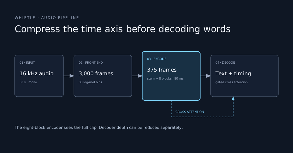
Whistle’s decoder has eight layers, but it can run fewer. Cactus says it trained every depth from two layers upward as a usable model and lets the caller select a depth with --audio-depth. The encoder always runs all eight blocks. Selecting a shallower decoder therefore changes the text-generation part of the cost; it does not shorten feature extraction or audio encoding. That distinction is important when estimating the benefit on a particular device.

The decoder searches five candidate transcripts and limits output to 320 tokens. It has 8,192 text pieces plus a token for each supported language, so the predicted language appears in the decoded sequence. Keyword biasing follows the supplied phrases during that search. These choices explain why the model can support multilingual transcription, word timing, and application vocabulary within the same runtime, but they also define limits: a single pass is capped at 30 seconds, and the text output has a finite token budget.

Reading the benchmark without overreading it

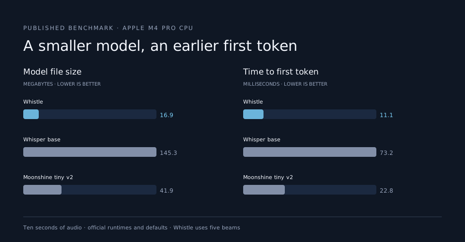
The headline comparison is striking. Whistle’s 16.9 MB file is about 8.6 times smaller than the 145.3 MB Whisper base model in the published comparison. On ten seconds of audio, Cactus reports an 11.1 ms time to first token for Whistle, 73.2 ms for Whisper base, and 22.8 ms for Moonshine tiny v2. Its reported post-first-token decode rates are 1,319, 266, and 262 tokens per second respectively.

Those numbers describe a specific test: an Apple M4 Pro CPU, ten seconds of audio, each model’s official runtime at its default settings, and Whistle using five beams. Time to first token starts when audio enters and ends when the first token appears; the decode rate divides generated tokens by time after that point. Neither figure alone is the duration a user waits for a complete transcript. The models also used different numerical precision and implementations. The comparison measures the packages as shipped in that setup, not equalized architectures running through one engine.

Word error rate tells a more mixed story than the speed chart. Cactus reports Whistle ahead of Whisper base on LibriSpeech’s clean and other splits, SPGISpeech, Earnings-22, and the average over its seven FLEURS languages. Whisper base is ahead on TED-LIUM, AMI, and the MLS average. Moonshine’s published results are English only, so missing multilingual bars are not zero-error results. Some figures also use different corpus subsets: the Whisper AMI number is AMI-IHM, while the others use a different AMI selection.

Cactus says it evaluated Whistle over 86,174 utterances and checked audio hashes and speaker IDs for overlap with training and validation material. Whisper and Moonshine error rates in the chart come from their authors’ publications. That is valuable context, but it means the comparison is assembled from published results rather than one independent lab rerunning every model on every corpus. Before choosing a model for a product, test your own accents, background noise, vocabulary, device class, and long recordings. An average error rate can hide exactly the names or commands that your application cannot afford to miss.

One runtime for speech and actions

Whistle shares Needle’s .cact container, quantization, CPU kernels, and C++ engine. An application can load Whistle by itself for transcription or load it beside Needle for tool selection. In the combined path, the engine accepts an audio clip, transcribes it, passes the text to Needle with the application’s tool schema, and returns a JSON object containing tool calls plus speech fields such as audio_text and audio_language.

That arrangement removes an application-level handoff between a speech SDK and a separate command model. It also keeps the transcript inside the local engine when the device runs both models. For a light switch, wearable, or robot, a compact single-runtime stack can be easier to package and operate than a chain of services. The tool call still needs ordinary application checks: validate its arguments, enforce permissions, and treat an uncertain recognition as a reason to ask the user before a consequential action.

The model card links the weights and documents the Apache 2.0 license. The Needle repository provides the source and Python interface. A simple local call looks like this:

import needle

result = needle.transcribe("clip.wav")
print(result["text"])

For an already prepared 16 kHz WAV or raw samples, the base cactus-needle install is enough. The project also publishes prebuilt targets for desktop, mobile, browser, WASI, and several smaller architectures. A target being listed is a packaging claim; practical latency, memory use, and microphone integration should still be measured on the hardware you intend to ship.

Whistle’s contribution is a concrete design point: a small speech model that gives developers transcription, word timing, embeddings, and a route to local actions from one engine. Its size and first-token results make that design appealing for edge devices. Its corpus-dependent accuracy results, 30-second single-pass window, and hardware-specific benchmarks make testing on the intended workload the next step, not an afterthought.